| Return to CONTENTS | September 2012 |
| Abstract: |
Is there an overriding principle of nature, hitherto overlooked, that governs all population behavior? A single principle that drives all the regimes observed in nature - exponential-like growth, saturated growth, population decline, population extinction, oscillatory behavior? In current orthodox population theory, this diverse range of population behaviors is described by many different equations - each with its own specific justification. We suggest that this collection of population behaviors all issue from a single principle. The signature of such an overriding principle would be a differential equation which, in a single statement, describes all the panoply of regimes. A candidate such governing equation is proposed. The principle from which the equation is derived is this: The effect on the environment of a population's success is to alter that environment in a way that opposes the success. |
1. Traditional Perspective
The acknowledged source of theories about population is the monograph by the venerable Thomas Malthus. (Malthus 1798) His place in history rests largely on these two sentences from page 4,
Population, when unchecked, increases in a geometrical ratio. Subsistence increases only in an arithmetical ratio. |
The archaic terms 'geometric ratio increase' and 'arithmetic ratio increase' are today called 'exponential growth' and 'linear growth'. In this quote he takes pains to distinguish these because his thesis is based on the distinction. Malthus was thinking only of human population. Darwin (Darwin 1859) took the idea to apply to populations in the whole animal and vegetable kingdoms.
The rationale for exponential growth is this: In living systems growth is proportional to the population because each member (or pair of members) once produced, begin, themselves, to reproduce. There are more reproducers in a larger population. So the greater the number in the population, the greater is the growth. The same for deaths. The rate is proportional to the number available to die. However, as will be demonstrated in the next section, this analysis is only superficially true. Because the proportionality is not constant the idea is fundamentally flawed.
Malthus didn't offer equations to express these thoughts but it's instructive do so. Call the number of members in the population, n. At each moment of time, t, there exist n individuals in the population. So we expect that n=n(t) is a continuous function of time.
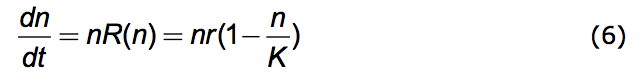
The rate of growth of the population is dn/dt; the increase in the number of members per unit time. That this is proportional to population number, n, is the substance of the idea. Call the constant of proportionality, R. Then the differential equation that embodies the idea of 'increase by geometrical ratio' is:
|
When R is constant, its solution yields the archetypical equation of exponential growth.
 |
The no is simply the starting population, no=n(0); the number of its members at t=0.
Again with R as constant and no as defined above, linear growth - not a solution of (1) - is expressed by this equation:
 |
These formulas for n(t) exhibit starkly different behaviors. That is why they were contrasted by Malthus.
Now, common experience tells us that exponential growth cannot proceed indefinitely. No population grows without end. Suppose the birth rate declines. Maybe, instead, the death rate increases. Perhaps because the weather got cold or food became scarce. Then this is accounted for by a new exponent, say R'; a smaller one. So R is no longer viewed as being constant. It may vary with time. R = R(t).
In describing living systems the idea has been to retain that fundamental exponential-like form and seek to explain events by variations in R. The problem of explaining and predicting the dynamics of any particular population boils down to defining how R deviates from the expectation of uniform growth
. (Berryman 2003) The concept is that exponential growth is always taking place but at a rate that varies with time. Put mathematically:
 |
Fisher endows R with its own name, the Malthusian Parameter. (Fisher 1930) Equation (4) is called Darwinian Dynamics by Michod. (Michod 1999) In connection with his writing on genotype fitness Michod's Fisherian Fitness
is exactly of this form. Equation (4) is a powerful analytical tool for assessing population data.
Of course, any theory on how R might depend on n - rather than on t - produces a theoretical R(t). This is because the differential equation:
 |
is completely solvable for n as a function of t. Once we have n(t) we can deduce R(t) via it's definition in equation (4). This theoretical R(t) may be compared to measurements of (1/n)dn/dt so as to assess whether the theory is verified.
An object example of this process is provided by the celebrated Verhulst equation.
 |
A population history, n vs. t, resulting from this equation is the black one of Figure 1.
What motivated Verhulst (Verhulst 1838) is the common observation that nothing grows indefinitely. Here the constant, r, is the exponential growth factor and K is the limiting value that n can have - the carrying capacity of the environment
.(Vainstein et al. 2007) The equation insures that n never gets larger than nMAX = K. Because n is understood to be the number in a given physical space it represents, in fact, a population density (number/space). That this density has a limit is the reason for the association of K with crowding. The name, r/K Selection Theory, derives from the competing dynamics of exponential growth and of crowding - the r and the K. The Verhulst (Logistic) equation is often embedded in research studies. (Nowak 2006; Torres et al. 2009; Jones 1976; Ruokolainen et al. 2009; Okada et al. 2005; Ma 2010)
2. Shortcomings of the traditional perspective.
The textbook mathematical structure outlined in the last section has acquired the weight of tradition. It is certainly appealing. But it has serious failings.
Assigning all behavior to variations in R seems to preserve the pristine Malthusian exponential growth idea. But, in fact, allowing R to vary with time severs the connection to exponential growth.
The idea is dramatized in this example. Malthus makes it clear that if a population is growing exponentially with time then it is certainly not growing linearly with time. Linear growth is the antithesis of exponential growth. Equations (2) and (3) display the difference. But suppose R varies as R(n) = C/n. Using this in solving the Malthusian Equation, (5), produces exactly linear growth! The constant C is noR. Linear growth is variable-rate exponential growth! 'Variable exponential' growth is not 'exponential' growth.
There is no more content in conjectures about R(t) than there is in theorizing directly about how n might depend on t; n = n(t). Except for the tenacity of tradition there is no reason to focus on R as the basic parameter of population dynamics. Because R(t) can be anything so, too, can n(t) be anything. An equation expressing a true principle of population dynamics would yield only those behaviors biologically and ecologically possible for n(t). Equation (4) doesn't do this. It does no more than substitute one variable for another.
A good reason not to use R concerns extinction. A phenomenon well known to exist in nature is the extinction of a species. ... over 99% of all species that ever existed are extinct
(Carroll 2006). But there exists no finite value of R - positive or negative - that yields extinction. There is no mechanism for portraying extinction. It cannot be represented by R except for the value negative infinity; -∞. So, in fact there is good reason to avoid R as the key parameter of population dynamics.
In the continuous-n perspective the mathematical conditions for extinction are n=0 and dn/dt < 0. No infinities enter computations founded on these statements. Hence embracing n(t) directly allows one to explore the dynamics of extinction.
Next consider the eponymous Verhulst Equation (the Logistic Equation). Verhulst's K doesn't derive from some fundamental biological constraint. It's motivated only by the observation that populations never grow to infinity. They are bounded. But there are other ways - not described by Verhulst's equation - in which population may be bounded. For example, n(t) may oscillate. Or, as in Figure 1, a curve essentially the same as Verhulst's may arise from an entirely different theory where no K = nmax limit exists. One of the possible population histories resulting from the alternative theory offered below - which contains no nMAX - is shown in blue. Data fit by one curve will be fit equally well by the other.
The limited validity of r/K Selection Theory has been noted by researchers over the years. (Parry 1981; Kuno 1991)
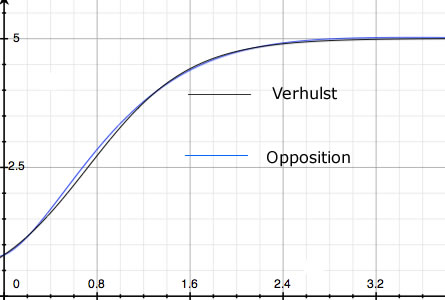 |
| Figure 1. Two population histories: number vs. time. The black curve is the Verhulst Equation. The blue curve is one of the solutions to the Opposition Principle differential equation. |
The most significant failing of the accepted Malthusian Structure of population dynamics is its limited domain of validity. Many population histories cannot be fit by exponential growth nor by the logistic equation. Oscillatory behavior demands that a new paradigm be requisitioned; the Lotka-Volterra equations (Lotka 1956, Volterra 1926) or, because their solutions are not structurally stable, their later modifications (Murray 1989, Vainstein et al 2007).
Thus, in current orthodox population theory, to describe the entire range of population behaviors requires many different equations - each with its own specific justification. Exponential growth has a limited range of validity, as does the Logistic Equation, and any other equation of first order. And none of these describe population oscillations, nor population decline, nor extinction.
No structure exists that embraces - in one single statement - all possible behaviors. Contemporary theory offers no overriding principle that governs the gamut of population behaviors. To produce such a structure is the aim of what follows.
3. The power of conceptual coalescence
Why is such an undertaking important? Because the purpose of science is to perceive the principles by which nature is governed. The methods of science uncover the facts of nature. But the greater mission of science is to see in those facts the principles governing nature. Progress in understanding is marked by conceptual coalescence: the quest to embrace an ever larger body of findings with ever fewer statements of principle. Paraphrasing Mark Twain, the task of science is to describe a plethora of phenomena with a paucity of theory.
Newton showed that the motion of things on earth are governed by the same rules as the motions of heavenly bodies. Formerly these two had appeared to be unrelated domains. He showed that a single principle governed them both. This synthesis was magnificently fruitful. It underlies our understanding of anything mechanical or structural. Much of our material well being depends on it.
Darwin's principle of natural selection explained a wealth of biological phenomena by a single idea. Through his synthesis the concept of evolution became part of our intellectual heritage.
Wegener showed us that continental drift - plate tectonics - is the underlying reason for such diverse phenomena as the distribution of fossils in the world, the shape of continents, earthquake belts and volcanic activity. That insight has proved remarkably beneficial.
Mendeleev gave structure to the chaos of chemistry with his table of the elements. He consolidated a profusion of chemical data into an all encompassing tabular statement of principle. This undertaking led to the understanding that matter was made of atoms. (Mendeleev, himself, never believed this!)
James Maxwell brought electricity and magnetism together by an overriding formalism that covered them both. The undertaking gave rise to an understanding of the nature of light.
Laws of Nature are not immutable. They may lose their status. This process of conceptual coalescence is an ever evolving one. Newton's laws on mechanical motion and Maxwell's on electromagnetism are incompatible. In 1905 Einstein produced a theory that embraced both of these vaste domains. In it Newton's principles become a limit behavior of a more all inclusive theory - relativity. So a law of nature can be dethroned - albeit still cherished and useful. It can be subsumed under a principle which embraces a larger domain of phenomena. The broader the scope of applicability the more valuable is the theory. Einstein's laws of nature absorbed Newton's. Relativity spawned nuclear energy, a deeper understanding of stellar processes and much more.
All of these examples have in common that a wide breadth of empirical observation is accounted for by a single idea. We see in them that conceptual coalescence is a foundation stone of scientific understanding. In that spirit, offered here is a candidate synthesis: a single differential equation that brings together the disparate domains of population behavior. We suggest that the panoply of population behaviors all issue from a single principle.
As long ago as 1972 (Ginzburg 1972), in a challenge to orthodox convention, L. R. Ginzburg took the bold step of proposing that population dynamics is better represented by a second order differential equation. All accepted formulations relied on first order differential equations as they still do today. He developed his thesis over the years (Ginzburg 1986, 1992, Ginzburg and Taneyhill 1995, Ginzburg and Inchausti 1997) culminating in the pithy and persuasive book, "Ecological Orbits" (Ginzburg and Colyvan 2004).
Perhaps the connection between conceptual coalescence and differential equations is best appreciated via a simple example.
Consider a fluid streaming steadily out of a spigot. Say from a tap in a beer barrel. The stream pours into a vessel; a straight walled cylindrical one where the level to which it's filled is visible. How does this level - call it L - change with time, t? Evidently the answer depends on details: the strength of the stream, the diameter of the vessel being filled and the amount of fluid initially contained in that vessel.
But one can describe, in one differential equation, all the possible answers to this question! All answers to what L(t) is. One may capture 'spoutness' (fluid streaming out of a spout into a container) in one statement and therefore in one equation. And from this one differential equation produce all the possible different curves of L vs t.
The equation is d2L/dt2 = 0.
It is the simplest second order differential equation imaginable. It says that, no matter the details, the core of the process is that fluid comes out steadily at a fixed volume per unit time. Therefore - whatever the vessel size or the flow rate or the fluid substance or the initial amount in the vessel - the fluid level height will increase at some constant rate - from any spout at all. That is what the differential equation says. It expresses a truth about spoutness. And using the rules of calculus one extracts, from this one differential equation, the curve describing any particular instance of filling.
Water flowing out of my household kitchen sink faucet is a particular instance. One of the myriad equations spawned by the foregoing differential equation represents it. L = (1cm/sec) x t. This equation's verbal translation is: in the originally empty vessel the level of liquid steadily rises with time by 1 centimeter every second when it's under the spigot.
Suppose the family of solutions to a single second order differential equation should match population behavior just as well as the many accepted first order equations do. That family of solutions have in common their single progenitor. Embedded in them is the principle that generated them.
When the family of solutions to a differential equation is found to fit empirical reality then that equation is expressing a truth about nature. It can give us insights and enable us to make predictions. Producing a second order equation whose solutions characterize a variety of population behavior is equivalent to uncovering a principle of nature governing those populations.
In the following we take a route different from Ginzburg's and arrive at a substantially different equation - albeit a second order one. We procede from a guess at what may be the underlying principle and then derive the second order differential equation that expresses that principle. If empirical reality is well fit by the progeny of that equation then we may conclude that the principle is true. And we will have produced a conceptual coalescence: a tool for better understanding nature.
4. Conceptual foundations for an overriding structure
We seek a mathematical equation to embrace all of the great variety of population behaviors. The equation is built on some foundational axioms. Empirical verification of the equation they produce is what will measure the validity of these axioms. The axioms are:
First: Variations in population number, n, are due entirely to environment.
Conceptionally we partition the universe into two: the population under consideration and its environment. We assume that the environment drives population dynamics; that the environment is entirely responsible for time variations in population number - whether within a single lifetime or over many generations.
The survival and reproductive success of any individual is influenced by heredity as well as the environment it encounters. This statement doesn't contradict the axiom. The individual comes equipped with heredity to face the environment. Both the environment and the population come to the present moment equipped with their capacities to influence each other; capacities derived from their past histories.
That the environment molds the population within a lifetime is clear; think of a tornado, a disease outbreak, or a meteor impact. That the environment governs population dynamics over generations is precisely the substance of 'natural selection' in Darwinian evolution.
That principle may be summarized as follows: ... the small selective advantage a trait confers on individuals that have it...
(Carroll 2006) increases the population of those individuals. But what does 'selective advantage' mean? It means that the favored population is 'selected' by the environment to thrive. Ultimately it is the environment that governs a population's history. Findings in epigenetics that the environment can produce changes transmitted across generations (Gilbert et al. 2009; Jablonka et al. 2009) adds further support to this notion.
Much productive research looks at traits in the phenotype that correlate with fitness or LRS (Lifetime Reproductive Success). (Clutton-Brock 1990; Coulson et al. 2006) The focus is on how the organism fits into its environment. So something called 'fitness' is attributed to the organism; the property of an organism that favors survival success. But environmental selection from among the available phenotypes is what determines evolutionary success. The environment is always changing so whatever genetic attributes were favorable earlier may become unfavorable later. Hence there is an alternative perspective: fitness, being a matter of selection by the environment, is induced by it and may, thus, be seen as a property of the environment.
Although, fitness, in some sense, is 'carried' by the genome, it is 'decided' by the environment. Assigning a fitness to an organism rests on the supposition of a static environment; one into which an organism fits or not. A dynamic environment incessantly alters the 'fitness' of an organism.
This is the perspective underlying the axiom that variations in population number, n, are due entirely to environment.
In this view, although birth rates minus death rates yield population growth they are not the cause of population dynamics; rather birth and death rates register the effect of the environment on the population.
Second: An increasing growth rate is what measures a population's success.
The 'success' of a population is an assertion about a population's time development; it concerns the size and growth of the population. A reasonable notion of success is that the population is flourishing. We want to give quantitative voice to the notion that flourishing growth reveals a population's success.
Neither population number, n, nor population growth, dn/dt, are adequate to represent 'flourishing'. Population number may be large but it may be falling. Such a population cannot be said to be flourishing. So we can't use population number as the measure of success. Growth seems a better candidate. But, again, suppose growth is large but falling. Only a rising growth rate would indicate 'flourishing'. This is exactly the quantity we propose to take as a measure of success; the growth in the growth rate. By flourishing is meant growing faster each year. That the rate of change of growth is a fundamental consideration in population dynamics has been advocated in the past. (Ginzburg and Colyvan 2005)
The 'success' of a population over, say, one year is the increase in growth over that year. A growth rate of 1000 new members per month at the beginning increases, say, to 1500 new members per month at the end of one year. This amounts to an population success of 500 per month per year (500/mo-yr). Should the growth rate decline in the next year from 1500/mo to 1200/mo then, in that year the population success would be negative, -300 per month per year. Figure 2 is a visual illustration of the relationship between the three variables, population, its growth and its 'success' for a hypothetical population history.
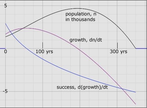 |
| Figure 2. A hypothetical population history, n = n(t); black curve. The population becomes extinct 350 years after it was first tracked from an initial 1300 members. It more than doubles in 200 years to reach a peak close to 5000 members. But its growth (purple curve) is zero at this population apogee. Then the population plunges precipitously - negative growth - going extinct after another 150 years. The success curve (blue) shows that the population was flourishing only in the first 60 years. Success is positive in those years. After that the seeds of decay appeared; the growth began to decrease. The population increased ever less rapidly until it stopped increasing altogether - at its apogee. At extinction, all of the parameters shown are finite even though R, at this point, is -∞. |
A corollary of these two foundational hypotheses is that change is perpetual. Equilibrium is a temporary condition. What we call equilibrium is a stretch of time during which dn/dt = 0. Hence 'returning to equilibrium' is not a feature of analysis in this model.
Another corollary is this: The environment of one population is other populations. It's through this mechanism that interactions among populations occur: via reciprocity - if A is in the environment of B, then B is in the environment of A. So the structure offers a natural setting for feedback. (Pelletier et al. 2009) It provides a framework for the analysis of competition, of co-evolution and of predator-prey relations among populations. These obey the same equation but differ only in the signs of coefficients relating any pair of populations.
5. The Opposition Principle: quantitative formulation
Based on the understandings outlined above we propose that an overriding principle governs the population dynamics of living things. It is this: The effect on the environment of a population's success is to alter that environment in a way that opposes the success. In order to refer to it, I call it the Opposition Principle. It is a functional principle (McNamara et al. 2009) operating irrespective of the mechanisms by which it's accomplished. In the way that increasing entropy governs processes irrespective of the way in which that is accomplished.
The Principle applies to a society of living organisms that share an environment. The key feature of that society is that it consists of a number, n, of members which have an inherent drive to survive and to produce offspring with genetic variation. Their number varies with time: n = n(t).
Because we don't know whether n, itself, or some monotonically increasing function of n is the relevant parameter, we define a population strength, N(n). Any population exhibits a certain strength in influencing its environment. This population strength, N(n), expresses the potency of the population in affecting the environment - its environmental impact. Perhaps this strength, N, is just the number n, itself. The greater n is, the more the environmental impact. But it takes a lot of fleas to have the same environmental impact as one elephant. So we would expect that the population strength is some function of n that depends upon the population under consideration.
Two things about the population potency, N, are clear. First, N(n) must be a monotonically increasing function of n; dN/dn > 0. This is because if the population increases then, surely, its impact also increases. Albeit, perhaps not linearly. Second, when n=0 so, too, is N=0. If the population is zero then certainly its impact is zero. One candidate for N(n) might be n raised to some positive power, p. If p=1 then N and n are the same thing. Another candidate is the logarithm of (n+1).
We need not specify the precise relationship, N(n), in what follows. Via experiment it can be coaxed from nature later. The only way that N depends upon time is parametrically through its dependence on n. In what follows we shall mean by N(t) the dependence N(n(t)). We may think of N as a surrogate for the number of members in the population.
The population strength growth rate, g = g(t), is defined by
 |
Like N, g too acquires its time dependence parametrically through n(t).
g = (dN/dn)(dn/dt)
To quantify how the environment affects the population we introduce the notion of 'environmental favorability'. We'll designate it by the symbol, f. It represents the effect of the environment on the population.
A population flourishes when the environment is favorable. Environmental favorability is what drives a population's success. We may be sure that food abundance is an element of environmental favorability so f increases monotonically with nutrient amount. It decreases with predator presence and f decreases with any malignancy in the environment - pollution, toxicity
But in the last section we arrived at a quantitative measure of success. The rate of growth of the population strength - 'the growth of growth' or dg/dt - measures success. Hence, that a population's success is generated entirely by the environment can be expressed mathematically as:
 |
By omitting any proportionality constant we are declaring that f may be measured in units (time)-2. Since equation (8) says that success equals the favorability of the environment, it follows that f measures not only environmental favorability but also population success. One can gauge the strength of the favorability of the environment - the value of f - by measuring population success.
We're now prepared to caste the Opposition Principle as a mathematical statement. The Principle has two parts. 1. Any increase in population strength decreases favorability; the more the population's presence is felt the less favorable becomes the environment. 2. Any increase in the growth of that strength also decreases favorability.
Put formally: That part of the change in f due to an increase in N is negative. Likewise the change in f due to an increase in g is negative. Here is the direct mathematical rendering of these two statements:
 |
We can implement these statements by introducing two parameters. Both w and α are non-negative real numbers and they have the dimensions of reciprocal time. (Negative w values are permitted but are redundant.)
 |
These partial differential equations can be integrated. The result is:
 |
The 'constant' (with respect to N and g) of integration, F(t), has an evident interpretation. It is the gratuitous favorability provided by nature; the gift of nature. Equation (11) says that environmental favorability consists of two parts.
One part depends on the number and growth of the population being favored: the N and its time derivative, g. This part has two terms both of which always act to decrease favorability. These terms express the Opposition Principle.
The other part - F(t) - is independent of N and of g. It is the gift of nature. There must be something in the environment that is favorable to population success but external to that population else the population would not exist in the first place. This gift of nature may depend cyclically on time. For example, seasonal variations are cyclical changes in favorability. Or it may remain relatively constant like the presence of air to breathe. It may also exhibit random and sometimes violent fluctuations like a volcanic eruption or unexpected rains on a parched earth. So it has a stochastic component. All of these are quite independent of the population under consideration. In fact, however, dF/dt may depend on population number since this is the rate of consumption of a limited food supply.
Inserting equations (7) and (8) into (11) we arrive at the promised differential equation governing population dynamics under the Opposition Principle. It is this.
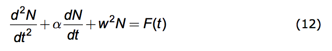 |
In the world of physical phenomena this equation is ubiquitous. Depending upon the meaning assigned to N it describes electrical circuits, mechanical systems, the production of sound in musical instruments and a host of other phenomena. So it is very well studied. The exact analytical solution to (12), yielding N(t) for any given F(t), is known.
6. Some consequences
To explore some of the consequences of this differential equation we consider the easiest case; that the gift favorability is simply constant over an extended period of time. Assume F(t) = c independent of time. Non-periodic solutions arise if α ≥ 2w. One of these, displayed in Figure 1, produces results similar to the Verhulst equation - the Logistic Equation. And like that equation they exhibit an exponential-like growth over a limited range.
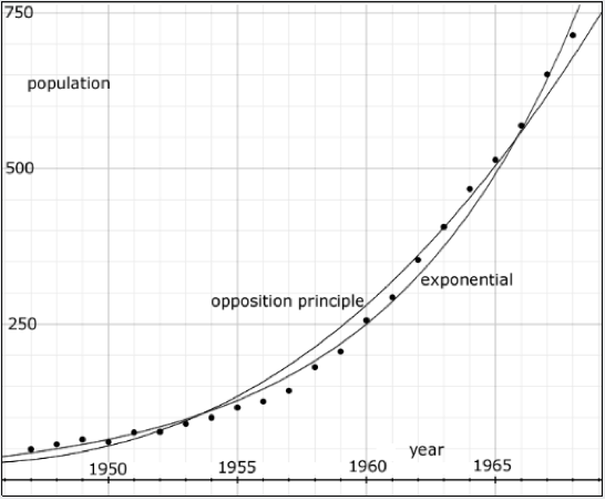 |
| Figure 3. Data points, gathered every year from 1947 to 1968, reporting the number of musk ox on Nunivak Island, Alaska. The curves show that both an exponential and an Opposition Principle curve may be fit to the data. |
Empirical data on such an exponential-like growth is exhibited in Figure 3 showing the population of musk ox (Ovibos moschatus) isolated on Nunivak Island in Alaska (Spencer and Lensink 1970). The data, gathered every year from 1947 to 1968, is in Table 1 of Spencer and Lensink's paper. It is, indeed, well fit by an exponential curve showing the formidable growth rate of 13.5% per year.
The population cannot possibly fit such a curve indefinitely. Nothing grows without end. The exponential curve fits the population data only in the domain shown. But, in this domain, the data is also well fit by an Opposition Principle curve where α = 0.02 per year, w = 0.0076 per year and n=N.
If α < 2w the solutions to (4.6) are periodic and are given by:
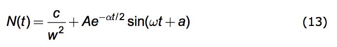 |
where the amplitude, A, and the phase, a, depend upon the conditions of the population at a designated time, say t=0. And the oscillation frequency, ω, is given by:
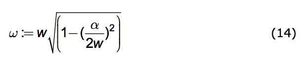 |
In Figure 4, equation (13) is compared to empirical data. The figure shows the population fluctuations of larch budmoth density (Turchin et al. 2003) assembled from records gathered over a period of 40 yrs. The data points and lines connecting them are shown in black. The smooth orange curve in the background is a graph of equation (13) for particular values of the parameters.
 |
| Figure 4. Observational data on the population fluctuations of larch budmoth density is shown as black diamonds and squares. The smooth orange curve is a solution of Equation (13). |
We assumed α is negligibly small so it can be set equal to zero. The frequency, ω is taken to be 2π/(9yrs) = 0.7per year. The vertical axis represents N. In the units chosen for N, the amplitude, A, is taken to be 0.6 and c is taken to be 0.6 per year2. The phase, a, is chosen so as to insure a peak in the population in the year 1963; a=3.49 radians.
Because the fluctuations are so large the authors plotted n0.1 as the ordinate for their data presentation. The ordinate for the smooth orange theoretical curve is N. Looking at the fit in Figure 3, one might be led to conclude that the population strength, N(n), for the budmoth varies as the 0.1 power of n. But the precision of fit may not warrant this conclusion.
The conclusions that may be warranted are these:
Considering that no information about the details of budmoth life have gone into the computation the graphical correspondence is noteworthy. It suggests that those details of budmoth life are nature's way of implementing an overriding principle. The graphical correspondence means that, under a constant external environmental favorability, a population should behave not unlike that of the budmoth.
Equation (13) admits of circumstances in which population extinction can occur. If A > c/w2 then N can drop to zero. Societies with zero population are extinct ones. (On attaining zero, N remains zero. The governing differential equation, (12), doesn't apply when N < 0.)
But the value of A derives from initial conditions; from N(t=0) and g(t=0). So depending upon the seed population and its initial growth rate the society may thrive or become extinct even in the presence of gift favorability, c. This result offers an explanation for the existence of the phenomenon of 'extinction debt' (Kuussaari et al. 2009) and a way to compute the relaxation time for delayed extinction.
The case explored reveals that periodic population oscillations can occur without a periodic driving force. Even a steady favorability can produce population oscillations.
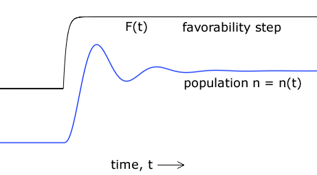 |
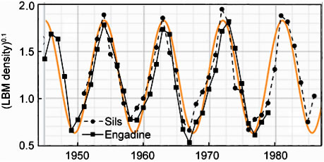
| Figure 5. A theoretical population history that can result from the Opposition Principle differential equation. |
Among the plethora of solutions to the governing differential equation, (12), is this one: Upon a step increase in environmental favorability - say, in food abundance - the population may overshoot what the new environment can accommodate and then settle down after a few cycles. Figure 5 illustrates this behavior. That there are such solutions amounts to a prediction that population histories like that of Figure 5 will be found in nature.
The data points (diamonds) of Figure 6 (Blount, Boreland, Lenski 2008) records the population of Escherichia coli (using optical density, OD, to measure it) maintained over 30,000 generations on a nutrient containing citrate which it could not exploit. Around generation 33,100 a mutation arose allowing a strain of the species to exploit this nutrient component. For those with this mutation the environment became suddenly more favorable and they flourished. Shown in the same figure is the theoretical curve arising from the Opposition Principle equation (13) with parameters α = 0.028 per generation and w = 0.023 per generation and n=N1.32.
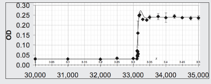 |
| Figure 6. Fit of Opposition Principle curve to the data on a strain of E coli for which, because of a mutation, a step increase occurs in the favorability of its environment. |
7. Conclusion
We noted at least five disparate regimes of population history - each with it's own individual and disjoint descriptive equation: exponential-like growth, saturated growth, population decline, population extinction, oscillatory behavior. It's argued here that these regimes can be brought under the embrace of a single differential equation describing them all.
That equation is the mathematical expression of general concepts about how nature governs population behavior. Being quantitative it offers us a framework with which to validate or refute these concepts. They are itemized as axioms and principles. Some of them run counter to accepted convention thus making empirical refutation a substantive matter. In short: a refutable proposition about the nature of populations is offered for assessment by the scientific community. Verification of the proposed equation would establish a basic understanding about the nature of living organisms.
References:
Berryman, A. 2003 On principles, laws and theory in population ecology. Oikos 103, 695-701
Blount, Z. D., Boreland, C. Z. and Lenski, R.E. 2008 Historical contingency and the evolution of a key innovation in an experimental population of Escherichia coli Proc. Nat. Acad. Sci. 105, 7899-7906
Britton, Nicholas F., 2003 Essential Mathematical Biology, London, Springer
Carroll, S. B. 2006 The Making of the Fittest. New York, NY: W.W. Norton
Clutton-Brock, T. H. (editor) 1990 Reproductive Success : Studies of Individual Variation in Contrasting Breeding Systems. Chicago, IL: University of Chicago Press
Coulson, T., Benton, T. G., Lundberg, P., Dall, S.R.X., Kendall, B.E. and Gaillard, J.-M. 2006 Estimating individual contributions to population growth: evolutionary fitness in ecological time. Proc. R. Soc. B 273, 547-555
Darwin, C. 1859 On The Origin of Species by Means of Natural Selection. London: John Murray
Fisher, R. A. 1930 The Genetical Theory of Natural Selection. Oxford: Oxford University Press.
Gilbert, S.F. and Epel, D. 2009 Ecological Developmental Biology. Sunderland, MA: Sinauer
Ginzburg, L. R. 1972 The analogies of the "free motion" and "force" concepts in population theory (in Russian) In V. A. Ratner (ed.) Studies on Theoretical Genetics. Novosibirsk, USSR: Academy of Sciences of the USSR, pp 65-85
Ginzburg, L.R. 1986 . The theory of population dynamics: I. Back to first principles. Journal of Theoretical Biology 122, 385-399
Ginzburg, L.R. 1992 Evolutionary consequences of basic growth equations. Trends in Ecology and Evolution 7,133; further letters, 1993, 8, 68-71
Ginzburg, L.R. and Taneyhill, D. 1995 Higher growth rate implies shorter cycle, whatever the cause: a reply to Berryman. Journal of Animal Ecology 64, 294-295
Ginzburg, L.R. and Inchausti, P. 1997 Asymmetry of population cycles: abundance-growth representation of hidden causes of ecological dynamics. Oikos 80, 435-447
Ginzburg, L. and Colyvan, M. 2005 Ecological Orbits. Oxford: Oxford University Press
Jablonka, E. and Raz, G. 2009 Transgenerational Epigenetic Inheritance: Prevalence, Mechanisms and implications for the study of heredity and evolution. Quarterly Review of Biology 84, 131-176
Jones, J. M. 1976 The r-K-Selection Continuum. The American Naturalist 110, 320-323
Kuno, E. 1991 Some strange properties of the logistic equation defined with r and K - inherent defects or artifacts. Researches on Population Ecology 33, 33-39
Kuussaari, M., Bommarco, R., Heikkinen, R.K., Helm, A., Krauss, J., Lindborg, R., Öckinger, E., Partel, M., Pino, J., Rodà, F., Stefanescu, C., Teder, T., Zobel, M. and Ingolf Steffan-Dewenter, I. 2009 Extinction debt: a challenge for biodiversity conservation. Trends Ecol. Evol. 24, 564-571
Lotka, A. J. 1956 Elements of Mathematical Biology. New York: Dover
Ma, Sam 2010 Did we miss some evidence of chaos in laboratory insect populations? Popul Ecol DOI 10.1007/s10144-010-0232-7
Malthus, T. 1798 An essay on the Principle of Population. London: J. Johnson
McNamara, J.M. and Houston, A.I. 2009 Integrating function and mechanism. Trends Ecol. Evol. 24, 670-675
Michod, R. E. 1999 Darwinian Dynamics: Evolutionary Transitions in Fitness and Individuality. Princeton, NJ: Princeton University Press
Murray, J.D., 1989 Mathematical Biology, Berlin: Springer-Verlag
Nowak, M. A. 2006 Evolutionary Dynamics: Exploring the Equations of Life. Canada: Harvard Press
Okada, H., Harada, H., Tsukiboshi, T., Araki, M. 2005 Characteristics of Tylencholaimus parvus (Nematoda: Dorylaimida) as a fungivorus nematode. Nematology 7, 843-849
Parry, G.D. 1981 The meanings of r- and K-selection. Oecologia 48, 260-264
Pelletier, F., Garant, D., and Hendry, A. P. 2009 Eco-evolutionary dynamics. Phil. Trans. R. Soc. B 364, 1483-1489
Ruokolainen, L., Lindéna, A., Kaitalaa, V. and Fowler, M. S. 2009 Ecological and evolutionary dynamics under coloured environmental variation Trends Ecol. Evol. 24, 555-563
Spencer, C. L. and Lensink, C.J. (1970) The Muskox of Nunivak Island, Alaska. The Journal of Wildlife Management 34, 1-15
Torres, J.-L., Pérez-Maqueo, O., Equihua, M., and Torres, L. 2009 Quantitative assessment of organism-environment couplings. Biol Philos. 24, 107-117
Turchin, P. 2003 Complex Population Dynamics: A Theoretical/Empirical Synthesis, Princeton: Princeton University Press
Turchin, P., Wood, S. N., Ellner, S.P., Kendall, B.E., Murdoch, W. W., Fischlin, A., Casas, J., McCauley, E. and Briggs, C. J. 2003 Dynamical effects of plant quality and parasitism on population cycles of larch budmoth. Ecology 84, 1207-1214
Vainstein, J.H., Rube J.M. and Vilar, J.M.G., 2007 Stochastic population dynamics in turbulent fields. Eur. Phys. J. Special Topics 146, 177-187
Verhulst, P-F., 1838 Notice sur la loi que la population poursuit dans son accroissement. Correspondance mathematique et physique 10, 113-121
Volterra, V. 1926 Fluctuations in the Abundance of a Species considered Mathematically. Nature 118, 558-560
March 2012
Marvin Chester
email
Return to Site Contents
11'09-
© m chester 2011 Santa Cruz CA